Niene Boeijen 900918-070-088 July 2015

Abstract

The amount of geospatial data is increasing rapidly. The magnitude and complexity of large geospatial datasets are a challenge to transform from information into knowledge. Geo-visualization is one of the tools to turn these heterogeneous data volumes into knowledge for a broader public. Also in the field of cultural heritage geo information systems is used more for conservation and safeguarding purposes. For cultural heritage the representation in the form of web-mapping is a suitable tool to make the data more open and promote heritage information. In this design oriented research an interactive web application is built to apply geo-visualization techniques to cultural heritage date sets. The case study is an area in Drenthe where field-names from the 18th century are collected. These field names tell us how the environment used to look, because they originate in the minds local inhabitants to navigate and communicate about their spatial orientation. The names often relate to landmarks and characteristics of the direct environment. Mostly, local altitude differences, vegetation and soil types. In the application the user is able to see the field names on a map and on a transect line, showing the relation of the field to the altitude of its direct environment. Through information texts, the user can relate the names to the characteristics of the surroundings. The goal is to preserve the living heritage of field-names, give the inhabitants of Drenthe the possibility to explore names that cannot be found in the real surroundings and turn the raw data that is only available to a small group of people, into knowledge for a broader audience about their landscape. The geo-visualization techniques were useful for the representation of the field names. Though every visualization of data needs a individual approach.

Keywords

Geo-visualization Heritage Drenthe Field names GIS

Abbreviations

AHN

Actueel Hoogtebestand Nederland

H&L

Heritage and Location Project

CH

Cultural Heritage

FIL

Future Internet Lab

GIS

Geo Information System

ICH

Intangible Cultural Heritage

RCE

Rijksdienst voor Cultureel Erfgoed

Introduction

Introduction

The amount of geospatial data has increased rapidly. Geospatial data is created and used increasingly every day in smart phones, digital maps, satellite navigation systems, websites, services and apps. Almost 60% of all data is geographically referenced. Next to that, the modern computer technologies provide better opportunities for institutions, organizations and citizens to create and use geospatial data. Already a wide range of domains, use geo information systems [GIS] for management and decision-making purposes and the fields of application are still expanding.(Cartwright, Miller, & Pettit, 2004; Hahmann & Burghardt, 2013; MacEachren & Kraak, 2001; Tensen, 2014)

The magnitude and complexity of data sets with geospatial reference are a challenge in information science. How to transform this data into information and subsequently into knowledge? Data is a product of research, creation, collection and discovery. It is raw material, often boring, incomplete or inconsequential. It is not yet valuable as communication, for it is not a complete message. (see figure 1). Often audiences are presented with data instead of information. According to Nathan Shedroff, successful communications do not present data. Communication is the process to get the story to the audience. Geo-visualization is one of the tools to turn large heterogeneous geo data volumes from information into knowledge. But geo-visualization to inform the general public is still in development. Geo-visualization integrates scientific visualization, cartography, image analysis, information visualization, data analysis and geographic information systems to provide methods and tools for visual exploration, analysis and presentation of geospatial data. (MacEachren & Kraak, 2001; Shedroff, 1999; Tensen, 2014)

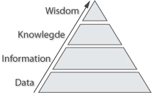
(Shedroff, 1999)

The web is being used to produce new visual applications, going beyond the status of maps and other representations of geographic information. The World Wide Web has become an extremely efficient channel for transferring data, and there is a need for creating user-centred geo designs to ensure that usable geospatial products are created and delivered. (Cartwright et al., 2004) This raises the interest for geo-visualization in publishing geo-referenced information on the web and getting the enormous amount of available data to the general public (Lin, Gong, & Wang, 1999; Tensen, 2014). Only a few methodologies specifically directed and web geo-visualizations emerge which emphasize the scientific information visualization techniques as a way to handle these very large and complex data sets. New visual forms and practices emerge, but how and why do they differ from the more conventional cartographic forms?

In this research, web geo-visualization is explored through a case study in the field of cultural heritage [CH].

Geospatial data and geo information systems provide big relevance for the field of cultural heritage conservation purposes. Safeguarding and exploiting CH is high on the agenda and includes the use of digital management systems. Before this was a hand-made task, but with the growing computer science there are new ways for the digital preservation, innovation and updating cultural heritage data. More and more central and local authorities responsible for cultural heritage use GIS as one of the main infrastructure components when digitalizing CH data. GIS systems provide a few possibilities; first, digitalizing CH data in a GIS system preserves the data, by presenting the digital records in the form of focusing on its relation to place. Geographical information systems have proved their potential to present and exploit cultural heritage data. Second, such a system can be used for research aims. Implementing analysis on the spatial correlation and relations of different datasets and enrich the knowledge already existing. (Droj, 2010; Karavia & Georgopoulos, 2013; Lai, Luo, & Zhang, 2012; Meyer et al., 2007) Lastly, by enriching current datasets by linking it in space and time to other datasets, which do not contain exact location data but do contain a sense of place in the thematic data description. Assumption is that the place referred to in historical documents probably refer to the identical real-world place if they are related in name. (Deal, 2014; Droj, 2010; Meyer, Grussenmeyer, Perrin, Durand, & Drap, 2007; Petrescu, 2007)

For cultural heritage data, the issue of the representation of the results of inventories in mapping systems and updating and maintaining the data, remains open. Web-mapping applications can be used to make open access-easy to use formats, for the assessment and promotion of heritage data. Web-mapping is a suitable tool for visualizing and updating geo heritage data. In general, much of the spatial data being created and shared is strongly visual in nature, including photographs, video, maps and art (Elwood, 2011; Martin, Reynard, Pellitero Ondicol, & Ghiraldi, 2014)

As stated by Deal:

Visualizations have the potential to greatly improve search and discovery for on-line collections, transforming how users interact with digital collections. Furthermore, changing technology is making it easier than ever to incorporate visualizations into search interfaces and websites. The time is ripe for cultural heritage institutions to begin experimenting with data visualization in earnest.

In the cultural heritage field, the temporal dimension plays an important role to explore data. (Cerasuolo, Cutugno, & Leano, 2012) Spatial-temporal data visualization assumes and important role in the data presentation to users. The three dimensional data form of geo data (spatial, temporal and descriptive) helps users understand and gain knowledge in the discovery process.

The goal of this research is to build a web-application to visualize geographically referenced intangible cultural heritage [ICH] data. There for this will be a design-oriented research. The context is a dataset of field names that were used by the local citizens around 1800 to refer to specific agricultural fields or areas, in Drenthe, the Netherlands. The information about the landscape that is hidden in the names gives a lot of historic information. Yet, noticeable is that this data is only known to a few selected historians. (Spek, Elerie, & Kosian, 2009) The data was supplied by the Rijksdienst voor Cultureel Erfgoed and based on the book “van Jeruzalem tot Ezelakker, levende veldnamen van de Drentse Aa”. More about the data will be described in chapter 2.1.

This research is part of an internship at Waag Society for the project of Heritage & Location. (see section 2.2.) This report describes the work and the results for the development of a web-application for the project Heritage & Location.

Objectives

The overall objective of this study is to build an attractive web-application for the project Heritage & Location to show its potential of visualizing intangible heritage data and preserving them. This will be done by using the case-study of field-names in Drenthe, the Netherlands. To achieve this, the following sub-objectives have been defined:

1. Establish design requirements and specifications for the prototype application that will be developed.
2. Develop a prototype version of the web-application.
3. Evaluate the prototype web-application according to the requirements from sub-objective 1.

Report structure

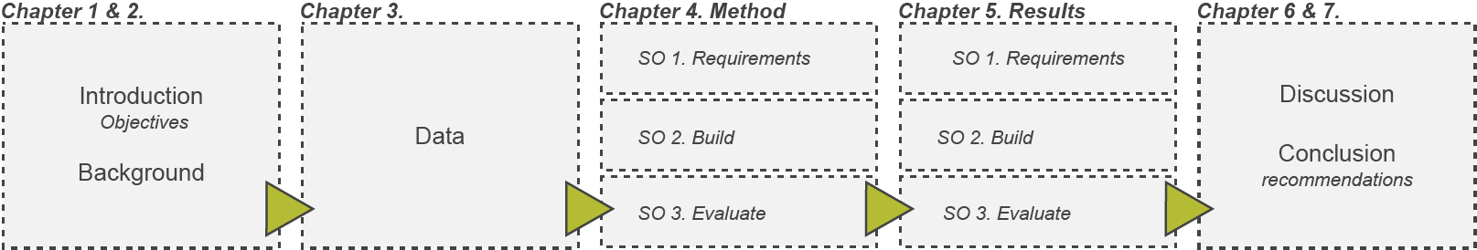
This report will exist of 7 chapters, including this introduction chapter. Explaining how the prototype web-application is established. The second chapter explains some concepts for background information. First, the field names will be explained as well as the background of the Heritage & location project from Waag Society. After this a summary of some geo-visualization techniques and frameworks will be given. This is composed as a reference for the design requirements and serves as inspiration for the design of the application.
The third chapter shows the field-name data provided by the RCE which forms the case study for this research. The fourth and fifth chapter provide per sub-objective, the methods and results. The last two chapters reflect on the findings and conclude the study as well as providing some suggestions and recommendation for further development. Figure 2 illustrates the structure of this report.

Background theory

In this chapter, the concept of field-names in Drenthe is explained and their position in the cultural heritage field. Because this research was conducted in the scope of the Heritage and Location project at Waag Society, this will also be elaborated on. After this, a summary of some geo-visualization techniques and frameworks will be given. This is composed as a reference for the design requirements and serves as inspiration for the design of the application. Starting with some static visualization forms, followed by dynamic and concluded with web-based interactive frameworks.

Field-names

A field-name is a toponym used for a small area of land or a certain surrounding. Mostly arable land, pasture lands, wastelands, uncultivated areas, hills, valleys, woodlands and swampy areas. The names are thought up by the local inhabitants for practical use in communication and spatial orientation. A field-name is often only existing in oral form and originates, develops or disappears while the environment changes. This makes field-names living heritage (see next section 2.1.1.) and it exist only in people’s memory. Therefore field-names fade away from daily lives and disappear with new generations. Written documentation of field-names date from the 17th, 18th and 19th century. Some names live through because they were taken up into official cadastre documentations or other landscape documentations. Nowadays, a new interest arises for field-names as they can tell us how the landscape used to look in the 18th century. Field-names contain words from landscape characteristics like which soil types, vegetation types or animals occurred. This link to specific landmarks or environmental characteristics tells us the origin on the name and tells us about how the landscape used to be. This information is highly important for nature conservation and heritage preservation. (Spek et al., 2009) They can be used for landscape design and planning, knowledge for historical research and inspiration source for artist. A collection of field-names was gathered by assessing people’s memories, old cadastre documents, maps and other collections. This mental map is now made tangible, by documenting as much as possible and digitalizing them into a GIS system. (Spek et al., 2009; Encyclopedie Drenthe Online, n.d.)

Intangible Cultural Heritage

The field-names in Drenthe are called living heritage, which is one of the 4 kinds of cultural heritage categories according to Volkscultuur institution;

1. The physical environment. Including monuments, archaeology sites and cultural landscapes.
2. Paper heritage; Stored in archives and libraries in the form of paper documents, maps and books.
3. Object collections, owned and displayed by museums. Only focusing on objects.
4. Living heritage; habits, traditions, religions and cultural events that people experience. From: (volkscultuur, nd)

Categories 1, 2 and 3 are tangible substances while category 4 is intangible heritage. UNESCO introduces the concept of intangible heritage data in 2003, to safeguard the importance of intangible cultural heritage and distinct it form tangible heritage and natural heritage. (UNESCO, 2003) Intangible cultural heritage can be shortly explained as all traditions and rituals of normal life, which gives people a sense of identity and continuity. ICH is transmitted from generation to generation and can be constantly recreated by communities due to interaction with their environment. (UNESCO, 2003; Zeijden, 2011) Intangible heritage is strongly depended on the features of space and influenced by the space. Of course these traditions, habits, etc., have a place where they take place. Or they are about a place, have a spreading, an origin, a continuation and can cover multiple places, through time. (Karavia & Georgopoulos, 2013)

This applies also for the field-names in Drenthe, which is oral living heritage. Originated with a strong influence of the direct environment it exists in.

Heritage and Location project

For this research takes place in the scope of the Heritage and Location [H&L] project at Waag Society, they both will be shortly explained.

Waag Society

Waag Society is an Institute for art, science and technology. They develop technical interventions for relevant social innovation. In 7 labs they conduct creative research in the form of projects; creative care lab, creative learning lab, future heritage lab, future internet lab, open design lab and open wet-lab. The Heritage & Location project (see next section 2.2.2) is part of the future internet lab [FIL]. The FIL focuses on the development of big and open data, making internet technology accessible and research the impact of the internet on society. (Waag Society, n.d.)

Heritage and Location

The project H&L is owned by the Rijksdienst voor het Cultureel Erfgoed [RCE] and at Waag Society in the FIL team, a historical-geo thesaurus and tools are developed. The H&L project aims to develop a uniform system to link CH collections to existing geometries, with the use of place indicators in the meta-data of the CH data. One of the tools is a historical-geocoder, to make heritage data, geo located and so link it in time and space to other heritage data sets and enrich knowledge. It combines multiple geo data sets with a time component and can be used easily to locate heritage data with a place notification. Big heritage collections with a place indication, though no geo data, can be linked to geometries. The goal of the H&L project is to know every place, administrative boundary, building and address that ever existed in the Netherlands. (Erfgeo, n.d., Erfgoed & Locatie, n.d.)

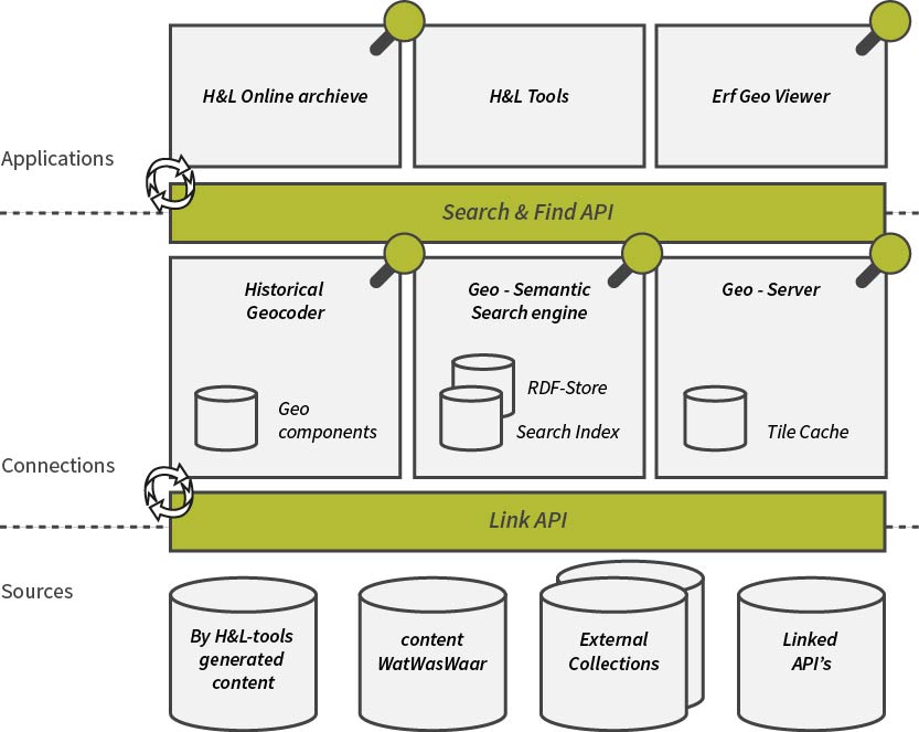
In figure 4 the overview of the H&L project is shown. Starting from the bottom with data sources, like cadastre maps, historical geo data and collections. This will be linked to the historical geocoder in a uniform way. So applications (top of the scheme) can easily search and find the geo data. Providing functions to search through time, location, bounding box, source, toponym etc. (Erfgeo, n.d., Erfgoed & Locatie, n.d.)

Examples of data that the geocoder contains are; old toponyms, disappeared villages, geometries of departments form 1830, urbanisation throughout the years, municipalities and their origin etc.

The data of the field-names can be regarded as a source of the H&L project. This has to be made uniform the system of the geocoder to eventually be able to build easy web-applications on top of the find API. This has not been done in this research for the project was not fully developed at the stage. For the future, the data might be taken up into the H&L project.

Geo-visualization

Geospatial data is data with a location, a connection to a location and oriented by their geographical relationships. Geo data has a nature of threefold: spatial, temporal and descriptive. The spatial dimension can be used to interpret the spatial dimensions and relation of data entities, an absolute and enclosed space wherein the geographic phenomena exists. The temporal dimension can be used to interpret the change in the data through time. The thematic dimension is to interpret what the data is about, a property that can be measured and assigned. The data component only concerns the raw observational data, with location, time and attributes. (Mennis et al., 2000; Nöllenburg, 2007)

Geo-visualization is a combination of communication, scientific information visualization, geographic information systems and cartography. It comes after the collection of data, transformations and analysis. See figure 5. From the real world we go to data and all the modifications to the data to eventually visualize it, either on a computer or on paper. The perception of people will interpret the data and turns the data into knowledge. In general, every map is a selective representation of reality and subjected to the interpretation of the human eyes. (Dibiase et al., 1992; MacEachren & Kraak, 2001)

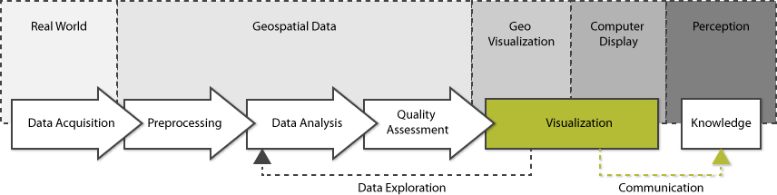
Geographical visualization can be used for 2 purposes; data exploration and information display. (Cartwright et al., 2004) By interpreting graphic representations new knowledge can be created and this can be distributed by visual communication. The one is exploratory, while visual communication is explanatory. (Dibiase, Maceachren, Krygier, & Reeves, 1992) In figure 5 the geo processing chain is combined with the series of visualization transformations, showing the position of visualization as exploration and communication.

In the following sections, some forms and frameworks of geospatial visualization will be explained. Starting to the first forms of static cartographic visualizations, to dynamic and animated maps. Eventually to web-based map, providing possibilities for interaction and user-centred designs.

Static geospatial visualization

Geo data has three basic symbols to represent the data; points, lines and polygons. Selecting the right graphic characteristic for data display is a challenging issue. Effective symbolization requires human creativity and judgement. The classic method for cartography is Bertin’s theory. This provides a classified system with four levels of data measurement and a list of graphic symbols that can be assigned to the visual variables. Bertin’s graphic variables are locations, size, density/size, texture, colour, orientation and shape. After Bertin, other researchers have added to this method with more graphic variables. Morrison added more specifications on colour, existing out of hue, saturation and value. MacEachren (1995) added the term clarity; build up from crispness, resolution and transparency. Caivano (1990) adds more dimensions on texture, defining directionality, size and density of texture.

Deciding the right graphic variable to be assigned to a certain type of data helps the viewer in defining the perceptual properties. For example, ordinal data needs the perception of being ordered, quantitative data of being proportional. While nominal data needs to be perceived as distinct categories. (Bertin, 2000; Caivano, 1990; Dibiase et al., 1992; MacEachren, 1995; Nöllenburg, 2007)

Bertin’s theory was designed in the context of static maps but is for a part the basis and seems applicable to the design of dynamic maps which require a set of dynamic graphic variables. Dynamic visual variables will only give the right results when combined with the traditional static visual variables. (Köbben & Yaman, 1996)

Dynamic geospatial visualization

A few forms of dynamic geo-visualization can be named:

• Display of time or spatial temporal visualization
• Animation
• Interaction

There are two categories of dynamic map display; temporal animation and non-temporal animation. In temporal animation, display time and world time are directly related. While for non-temporal, no direct relation between display time and world time is present. Kraak and Klomp give a slightly different categorization then Köbben & Yaman. An overview of the possible forms is shown in table 1. (Dibiase et al., 1992; Köbben & Yaman, 1996; Nöllenburg, 2007)

Categories of possible animations for dynamic phenomena.

Köbben & Yaman		Kraak & Klomp
Temporal	Direct relation between world time and display time	Time-series	World time
			Aggregated time
			Database time
Non - Temporal	No direct relation between world time and display time	Successive build-up
		Changing representations

Information from (Köbben & Yaman, 1996; Kraak & Klomp, 1996)

Also the dynamic categories can be divided into 2D and 3D animations. In this research we only work with 2D animations because of limited technology. Also in the theoretical frame work we will leave this out of consideration.

Spatial temporal visualization and animation will be explained in the following sections. Interaction will be combined with web-based visualizations, for interaction is the key aspect of web-based maps.

Dynamic variables

Dynamic visualization variables are identified by Dibiase et al. (1992), MacEachren (1994), Köbben and Yaman (1996), and Blok (2000). Dibiase states that dynamic variables can be used to emphasize the location of a phenomenon, emphasize the attributes or visualize change in the spatial, temporal or thematic dimensions. (Dibiase et al., 1992) Blok provides a framework for animated representation of dynamic geo-spatial phenomena. (Blok, 2000) They provide a range of dynamic visualization variables to be used for monitoring purposes of spatial temporal relationships and communication purposes of visualization.

Starting with no change vs change. Change can happen in the spatial domain, the temporal domain or the thematic domain of the data.

Categories of possible animations for dynamic phenomena.

Change in domain	Variables	Dimensions
Spatial	Appearance/disappearance	Born and Die
	Mutation	in size or shape
		increase/decrease (interval ratio)
		grow, shrink
	Movement	along trajectory
		boundary shift
Temporal	moment in time
	Pace
	Duration
	Sequence
	Frequency
Thematic	Mutation
	Thematic change

Animation

Animated maps use time to add a visual dimension to the display. The scenes in an animation show the state of the data at one moment accordingly. Animation is a form of spatial-temporal visualizations and contains the two categories; temporal animation and non-temporal animation. Animated maps contain dynamic variables such as scene duration, rate of change, scene order and contain hardly any interactive control. (Köbben and Yaman; MacEachren; Ormeling, 1996)

Dynamic animated variables are:

• Temporal position, when something is displayed.
• Duration. how long is something displayed.
• Order, the temporal sequence.
• State of change.
• Frequency or speed.
• Synchronization.

Web based geospatial visualization

With the emerging of web-based maps, the user is no longer depended on what the cartographer puts on the map. (Ogao & Kraak, 2002) With electronic maps, the user can navigate and explore the spatial data themselves with the given functionality. In a dynamic interactive visualization, the user pends between data presentation and exploration. (Ogao & Kraak, 2002)

Knapp (1995) defined four visualization operation tasks to be considered for web-based maps; identify, locate, compare and associate. Identify is describing an object, locate indicates the search for an object whose identity was already know. Associate and compare is the ability to relate between two different objects.

To cover the four visualization operations the user interface for a web page should have the following basic components:

• Geo browser – the map. Spatial dimension. Let users navigate.
• Time bar – temporal dimension.
• Filters – selecting information, filter. Thematic dimension.

For making the map, web map software is needed to create a map in the browser. Here some possible web map frameworks will be discussed as a foundation for further decisions made in the methodology. Widely known map frameworks are OpenLayers, MapFish and Leaflet. (Steiniger & Hunter, 2013)

OpenLayers is a library for WMS (tiled layers) and WFS (vector layers). It implements a JavaScript API for visualization of spatial data in the web browser. Without a server-side component. (Steiniger & Hunter, 2013) (http://openlayers.org/)

MapFish, is an open source web mapping framework for building rich web-mapping applications. MapFish provides specific tools for creating web services that allows querying and editing geographic objects. (Steiniger & Hunter, 2013) (http://mapfish.org/)

Leaflet is a web-map service WMS, that returns geo-referenced rasterized maps or tiles. In this context a map is considered a two-dimensional visualization of features in the common formats jpeg or tiff. Leaflet is open-source JavaScript library for interactive maps. (http://leafletjs.org)

Interactive geospatial visualization

Interactivity is one of the key aspects of web-based geo visualization. A map is nowadays seen as an interactive interface. Interactivity lets the user explore the geo-data and be in control and not depended on the cartographer. Interaction empowers the viewer/user to modify the data display. (Dibiase et al., 1992; Nöllenburg, 2007; Ogao & Kraak, 2002)The full potential of interaction in geo visualization lies in linking multiple views of the same data on the screen. Interactive visualization gives the control of the animation to the user, they engage in sorting, highlighting, filtering and transforming, the level of detail displayed and the speed can be determined. So information is less likely to be missed. Also called, guided discovery.

Two main interactive visualization techniques are introduced by Buja et al. from Nöllenburg (2007).

Focusing individual views. The user can modify the single display and what is seen. Choose the perspective, magnification level and level of detail. For example a set of navigation controls can be provided to zoom, pan and rotate. Layers can be selected to display or different attributes can be available to choose from. (Nöllenburg, 2007)

Linking multiple views. Linking means simultaneous highlighting of data items in multiple views in possible different formats. This can be combined with brushing; selecting display objects by pointing on them or encircling them on the screen. This stimulates visual thinking because data can be displayed in different ways and be analysed from different perspectives. The number, type and arrangements of the different views depend on the task, the user and the available space on the screen or specific interface. (Nöllenburg, 2007)

User centred geospatial visualization or Customer engagement

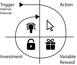
To engage the target group into an application the hook model will be explained. Figure 6. This models explains how a user can become addicted to an on-line product. First there is a trigger, to make the user want to use the application. This could be either an external (e-mail, advertisement) or internal trigger. When using the product, the user can makes actions for which they have to be rewarded. If users invest in the system they will likely stay and keep using the system, for they already put time and effort in that particular system. With multiple rewards and investments the user will go through the process again, for they get internal triggers to perform more actions.

The Data

From the Rijksdients voor Cultureel Erfgoed of the Netherlands a dataset with living field-names in Drenthe was supplied. This data contains field geometries that have a field-name, a name or toponym given to the plot or area by the people living in the neighbourhood from around 1830. These field-names were derived from studies by Naarding and Wieringa, together with het Drenthse Archief and het Meertens-Instituut. Old toponyms on old maps, tell us a lot, but here they used another source; the memory of the local inhabitants, where generation after generation the field names keep on living. The polygons where drawn by hand or the names were assigned to plots from the cadastre maps from 1830.

The most important factors influencing the forming of field-names are; natural relief, natural water and the vegetation structure. (Spek et al., 2009)

Further reference about the field names in Drenthe can be found in the book “Van Jeruzalem tot Ezelakker, Levende veldnamenatlas van de Drentse Aa”. (Spek et al., 2009)

The datasets contain in total 1747 polygons with a field-name. Projection RDNew. EPSG28992

This results in the following coverage of field names:

Field-name Amounts per source

Amount	Source
459	cadastre topographic map from 1832
452	Lanjouw
278	Wieringa
18	Kadaster
515	Drents Archief

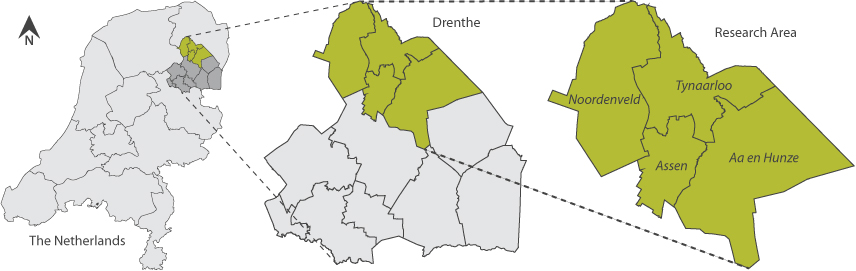
Based on this the total research location is determined, consisting of the municipalities Aa en Hunze, Assen, Noordenveld and Tynaarlo. All located in the watershed of the Drentse Aa.

Some of the field names are categorized in a previous study by the RCE. The category explains the origin of the name, specifically; which environmental characteristic was of the most influence on the name creation.

Method

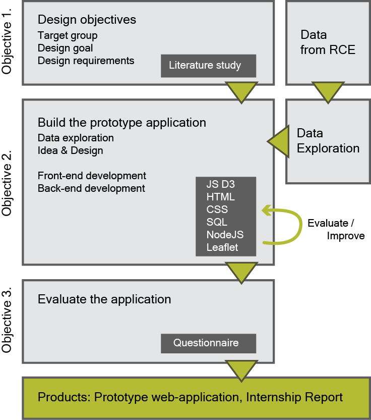
This research will be a design-oriented research. See figure 9 for an overview of the working procedure and where the specific objectives are addressed. First the design objectives are defined for the prototype application (objective 1). With the data provided by the RCE a small data exploration will be conducted to form an idea and make a design. This will process will be more iterative and chaotic then the overview shows. For design, exploration and requirements emerge in a mixed process. The main focus will be building the prototype application. (objective 2). Both the front-end and back-end design will be done by the conducting researcher as part of a learning experience for the internship project. In the end the prototype will shortly be tested to evaluate the design objectives from sub-objective 1. (objective 3)

The total time span of the project is 4 months, in which the research was set-up, executed and documented. Most creative choices and decisions will be taken by the researcher and her preferences.

Method Sub-objective 1. Finding the design requirements.

Analysis of users, task and context. Identification of requirements Design and prototype Test and evaluate

A literature research is done into geo visualization techniques and already available methods. Going from the conventional cartographic techniques to the modern techniques. Including animation and change. Also literature about building geo-web applications and the available techniques will be consulted. To add knowledge and experience from preceding researches to the development of the design requirements. This can be found in chapter 2. Background theory

A design oriented research contains several kinds of objectives, of which the following will be set. Based on personal preferences, supervision advice and expert advice from the internship colleagues.

• Define the target group
• Define the overall design goals
• Functional requirements
• User requirements
• Contextual requirements
• Assumptions (user, context, functional)

(Verschuren and Hartog, 2005)

Method Sub-objective 2. Building the prototype web-application

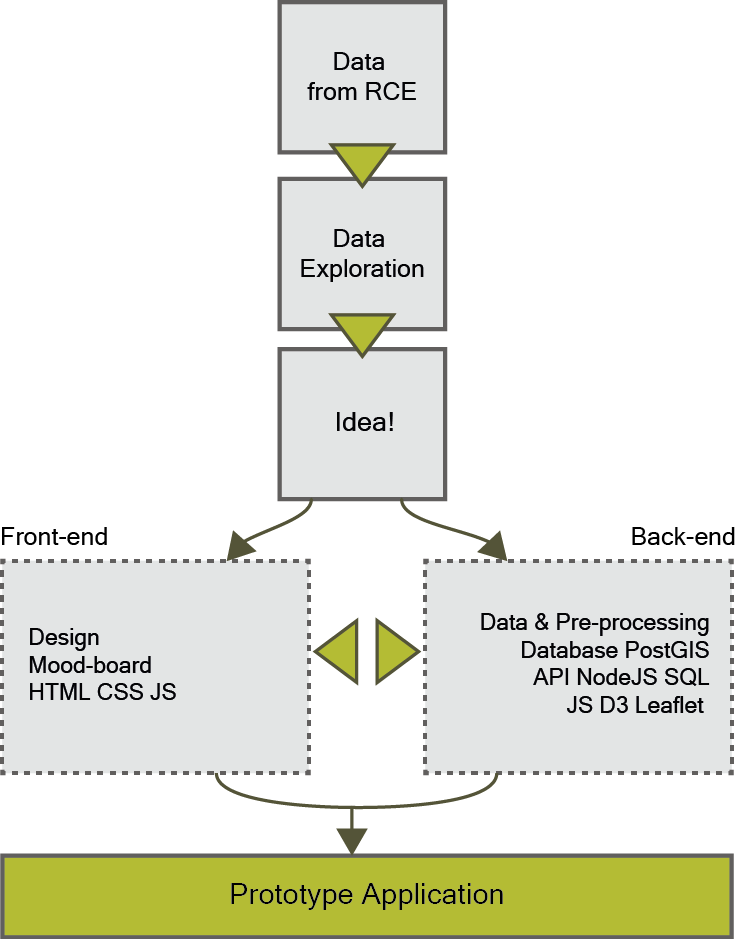
In order to build a prototype the design requirements have to be translated to a design. Figure 10 shows the steps that will be taken in order to develop the application.

First the data will be explored, to get an idea of the field-names. Also the literature provided with the field-names will be used to learn more about them. From this several ideas will be produced and the best will be chosen to continue with. Decisions and choices will be made on the personal preferences and experiences of the researcher and her supervisors.

When the idea is settled a front-end and back-end situation for the application have to be developed. Both will be developed by the researcher. Decisions and choices will be made on the developed goals and requirements, the background theory, personal preference and experience knowledge of supervisors.

The front-end is the presentation layer, so the web-page. A product of HTML, CSS and JavaScript for the web application so that a user can see and interact with it directly. The back-end is the data and data access layer of the application. The products will be a database, an API and the pre-processed data.

Eventually this will all from the prototype-product of this research.

Data exploration

Before the data could be explored it first had to be pre-processed a bit. When all data was complete and showed a good coverage of the area and the field-names, a search into possible interesting visualizations was done.

All the field-name data was delivered in separate .DAT files and scattered over several folders and sources. In order to work with the files in Qgis all the files needed to be converted to shape-files. This was done in R. In Qgis, manually the attribute names needed were changed in one standardized name in order to merge all the data together.

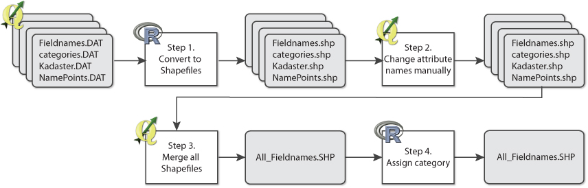
For scripts see the appendix 1, 2 and 3.

After merging the datasets it resulted into a lot of overlapping areas, so instead, the field-names were all linked to the Kadaster dataset from 1830. Now a single layer of polygons with multiple names is the result. This was done by spatially joining the datasets, or joining by the Kadaster ID’s which most of the datasets contained. The ID contained; municipality, sheet map number, parcel number.

Eventually, the field-names that had no category assigned, in the previous research by the RCE, had to be classified as well. This to have more coverage and amount of field-names.

The classification was done in R. See appendix 3 for the script. A field-name can consist out of multiple words with a different meaning and multiple categories and lemmings can be assigned to one field-name. The classification provided by the RCE was used. This contained per category, different codes and alternative words that signifies the same.

The script runs through all the field-names and all the possible categories, to match which category was applicable. These categories are given in table 4 with the amount of classes before and after the classification in R. In the appendix 4 a total overview of the categories and the names and alternative names can be found.

Field-name categories

Code	Category	Count old	Count new
A	Altitude	116	1109
B	Soil type	79	551
C	Water related names	33	199
D	River valleys and swamps	270	926
E	Forest	175	3146
F	Drift-sand fields	59	223
G	Wild animals	38	181
O	Miscellaneous	0	85
W	Wind direction	0	165
Total		770	6585

After this, in Qgis several names and possibilities were explored. Looking into combinations of categories, locations of specific names and this in relation to the height, water bodies, locations of build-up areas and land-use type.

The Idea

From one of the possible findings of the data exploration the main idea will follow. This is made on personal preference, no test were done for this.

Front-end

For the front-end development the following programming languages and packages were used:

• JavaScript
• HTML
• CSS

JavaScript packages needed for building the geo-application will be Leaflet. Leaflet is a JavaScript library for the creation of interactive maps by the founders of OpenStreetMap. D3.js will be used for the interactivity; this is a graphic drawing package.

Leaflet currently compete with OpenLayers only with respect to the display of map tiles, because OpenLayers offers much more functionality when it comes to interactive and vector-based map- ping tools. Also MapFish provides much more capabilities. For this was not needed for this application, the choice was made for using Leaflet, being light and simple.

Leaflet also has the applicability to install plug-ins. The MiniMap plug-in lets the user change the background map, and Leaflet Draw enables the creation of lines, polygons and points by the user.

See appendix 5 for the Leaflet map initializing code.

Back-end

First both client side and server side are built on one computer as a single seat set-up, in order to develop and test the processes. Once the desired result is achieved, the prototype application will be moved to a server with a database.

Database

The open source database PostgreSQL was installed with a PostGIS extension to create the needed database. It is currently the most popular free and open source spatial database (Steiniger and Hunter 2013). The PostGIS extension enables geographic objects like shape files and rasters.

First, the data needed for the application was downloaded and pre-processed. appendix 6 and 7 shows the pre-processing for the AHN2 data and the water topologies. The AHN2 tiles covering the research area were downloaded from nationaalgeoregister.nl to show the relation of the field-names with the environment. The water bodies are downloaded from the open data PDOK.nl. The Top10NLactueel contains all topology of the Netherlands on a scale of 1:25.000. Only the water bodies were used.

After pre-processing all the data was loaded in the database with a Dutch projected coordinate system RD new (EPSG:28992) See appendix 8 for the Shp2psql and Raster2psql lines used.

API

An API or application programming interface is needed to connect the web-application with the data in the PostGis database. For this purpose Brianc Node-Postgres is used. Node-Postgres is a PostgreSQL client for node.JS with pure JavaScript bindings.

For more info see:

• https://github.com/brianc/node-postgres
• https://nodejs.org/about/

See appendix 9 for the API request and response lines. The request makes use client response on Leaflet Draw. The response is send back to JS and handled with D3. Because Leaflet projects in WGS84 (EPSG:4326) the SQL query translates the coordinates to RDnew for intersection with the data in the database. In the end of the SQL query, it transforms it back to WGS84 in order to project the line correctly on the leaflet map again.

Method Sub-objective 3. Evaluating the web-application

A small test will be held to see if the product complies with the set goals and objectives. During the whole process, iteratively the web visualization was adjusted and tested again until the project ends.

The final test will be conducted with a small questionnaire. About 20 people will be asked to open the web-application and look at it, use it and play around with it. Afterwards, 8 statements will be given and asked to rate them to the level of agreeing or not. Ranks between a number of 1 and 5, from totally disagreeing till, total agreeing. Because the objectives were used in defining the statements, it tests if the application lives up to the objectives set for the user.

Because there is not an official testing group available, the participants will be colleagues of the Waag Society, the heritage institutions of the Heritage and Location project and possible, classmates and/or family and friends. This to have a broad general public.

Table 5 shows the statements asked and the connection with the design requirements which are in chapter 5.1 The complete questionnaire can be found in appendix 10.

Questions and Objectives

Number	Objective	Statement
1	U1	I think the application is visually appealing.
2	U2, U3	I feel tempted to use the tools and functions in the application multiple times.
3	U3	I feel tempted to use this application multiple times (in the future)
4	U4	The meaning and origin of the field-names became clear to me.
5	U5	The shown information is surprising and interesting.
6	U6	By using this application I understand more about the importance of safe-guarding the field-names as cultural heritage.
7	F1	The application is simple to use.
8	F2	Everything was working as I expected.

Results

Results Sub-objective 1. The design requirements

The main goal of this research is to build an attractive web-application for the project Heritage & Location to show its potential of visualizing heritage data and preserving them. A big part of the web application will be a geo-visualization of the intangible cultural heritage data set of living field names from Drenthe. The interactivity of the web application, will give users the possibility to discover the names in relation to the environment. The focus is on revealing hidden meaning of the raw data, for the general public.

Showing the field-names in an interactive application is explanatory visual communication. The goal of the field-names is explanatory, while the interactivity makes the data exploratory.

Target group

The target group will be defined as the common citizen, living in Drenthe and show an interest in their direct environment and want to discover something about its history. It will not specifically be targeted at children or elderly but to a general public. The target group’s language is Dutch.

Design goals

-G1 The goal is to preserve the living heritage names of Drenthe, which are mostly stored in people’s memory and so will disappear. -G2 Give the target group the possibility to explore them discovers them. For names cannot be found in the real surroundings, only in peoples memory and now given a place to exist. -G3 Getting the stories out of the raw data and show the target group the surprising knowledge that stays hidden. Help, the target group explore intangible cultural heritage and so the history of the Dutch landscape. Engage the target group in something interesting about their own landscape.

User requirements

The target group must feel:

• U1 Attracted to use the application
• U2 Attracted to stay and play around with the application
• U3 Challenged to explore more
• U4 Discover the meaning of the field-names in relation to their environment
• U5 Discover interesting stories and surprising facts about the field-names
• U6 Understand the field-names and their value

Functional requirements

• F1 The application must be intuitive and simple to use, so it shows quick and surprising results on the actions of the target group.
• F2 The application must be technically working in an efficient and error-safe way.

Context requirements

• Only free and open source software is used.

Assumptions

• The target group shows interest in the history of their living environment.
• The data from the RCE is a reliable source.

Results Sub-objective 2. Building the prototype web-application

Data exploration

In order to visualize the relation between the field-names and the geographical surroundings, several ideas came up to do this. As many characteristics are of influence, many possibilities could be chosen. The following ideas were shortly explored:

• Showing soil related field names on a soil map. A current or historic soil map.
• Showing height related field names on a height map.
• Showing ground water levels in relation to field names about water, swamps and soil types.
• Vegetation types, present on a field in the current situation vs what the field-name tells us about the historic vegetation.
• Showing names with relation to wind direction, in their position relative to the closest town or city.

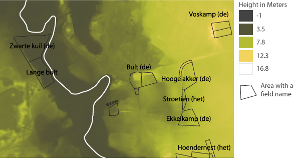
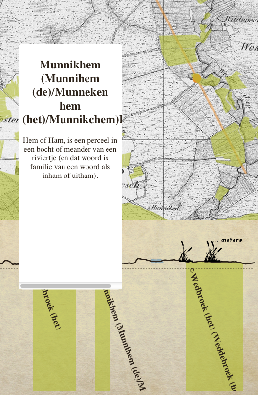
Figure 12 shows some fields with names related to height. Some fields do indicate small increases or decreases in the in relation to the area around. The Bult and the Hooge Akker are clearly on higher ground then the fields to the West. Where de zwarte kuil indicates that it is a lower field.

The idea

For the names are human invented they only reach as far as the naked eye could see. The relation of a field with a name can only be shown in relation to the direct environment. For example, a name like Bultakker (bump field) tells us that this field lies higher than its surrounding fields, not what the exact altitude it is. Therefore the main idea will be;

Showing the field names in relation to the height. By doing this, it includes names related to altitude, but also water and swamps, for lower areas are more wet then higher areas. Also vegetation type related names, will show correlation for this often depends on wet or dry situations and soil properties created by altitude differences.

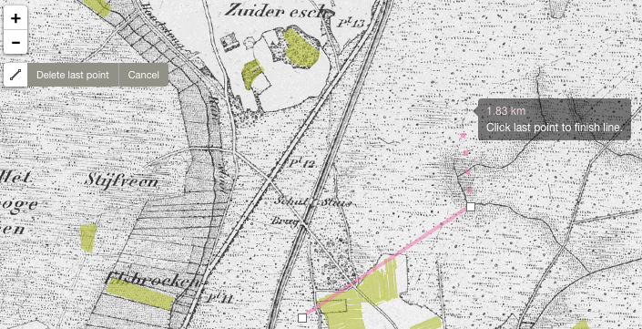
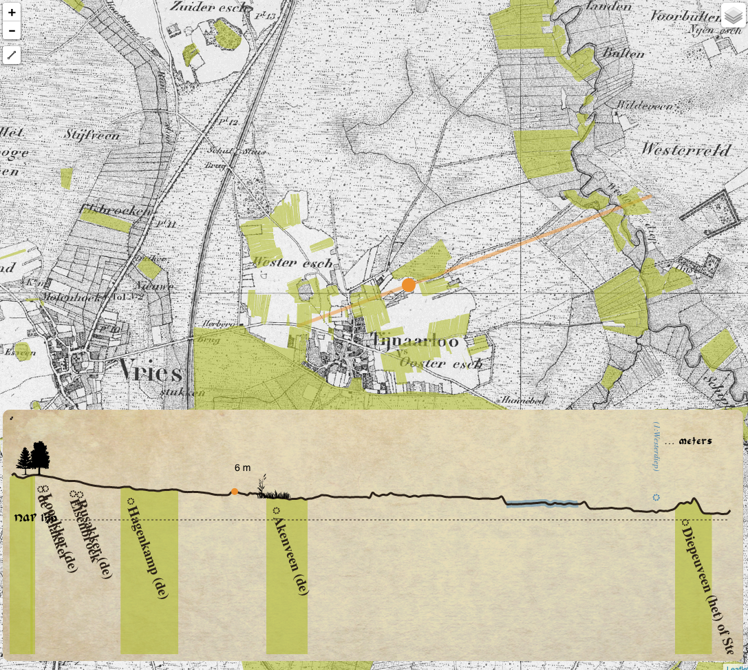
In order to include this in the visualization, showing the polygons on a map won’t be sufficient. Chosen is to draw a transect of the height data and indicate the names of the fields on this. The field-name data sets are static data, but will be displayed dynamically and interactive. It will let the user explore, and re-discover the information themselves, called guided discovery. (Nöllenburg, 2007)

The information will first be shown on a simple map and then in detail on a transect map. So the same information is shown in multiple views and from different perspectives. (linking) See section 2.3.4 .

The static display of the field-names will be on the map as simple polygons, to indicate their position and show the user the spatial dimension, the location and sizes of the fields. There will be a set of navigation controls for the map available to the user. Also multiple background layers form which the user can choose for extra information. The different base maps show the difference between 1830 and now.

The field names are historic but do not contain a change in time. Therefore the time bar had no relevance in the application.

Interactivity will be added to the transect line, letting the user define the transect line themselves and explore the different objects located on and around the transect line. The transect line, shows the relation between height, vegetation types on certain heights and the distance to rivers in accordance to the field-names.

Mouse-over actions will show information and stories about the origin of the names adding to the knowledge of the field-names and the environment. The brushing technique (section 2.3.4) will be used to highlight the height on the line and the position on the map of that specific point so the user can link between the two presentations.

Mood board

For the layout, ideas and colour use a mood board was made. Including inspiration pictures from the Internet. Search terms used are: living heritage, cultural heritage, transect and old transect map One of the main inspirations was the following image:

*Source: https://commons.wikimedia.org/wiki/File:1832_Erie_Canal.jpg *

Complete mood board; see appendix 11.

Custom fonts were explored to add to the feeling of an old map to the design. Old font was tried but made the names hard to read. So changed back to an easier to read font. Website used is www.fontsquirrel.com

Front-end

The result is a web-page with a geo-visualization. Including:

1. A map showing the area, where a line can be drawn to locate the position of the transect line. With navigational and drawing functionalities for the map.
2. A graphic transect line that can be explored. Including information about the field-names.
3. A panel showing the information about the field names.
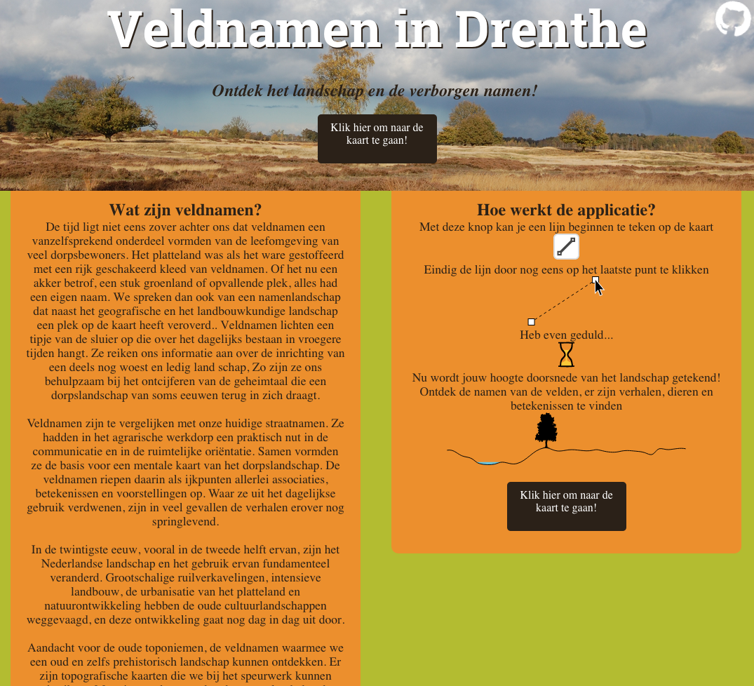
4. An opening page with explanation about how the application works.

The web application can be found on: maptime.waag.org/veldnamen .

Some screen-shots of how it looks. The first figure 14 is the welcome screen. Where information about the field-names is given and the explanation of the how the application works. If the user is ready they can press the button, to go to the map and start the application.

The next figure 15 shows how the screen looks when entering the application. An example line is already given to show the user what is possible.

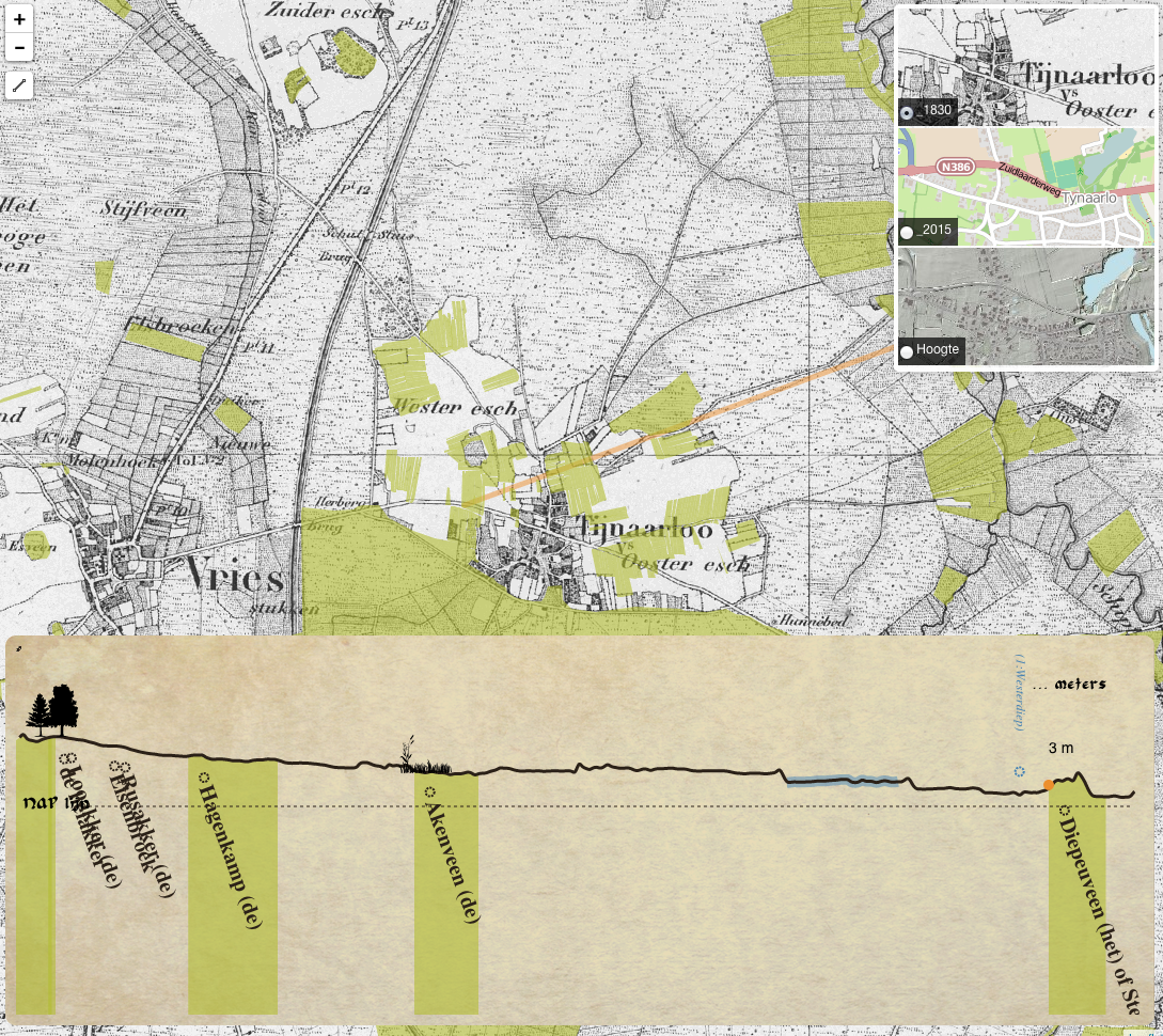
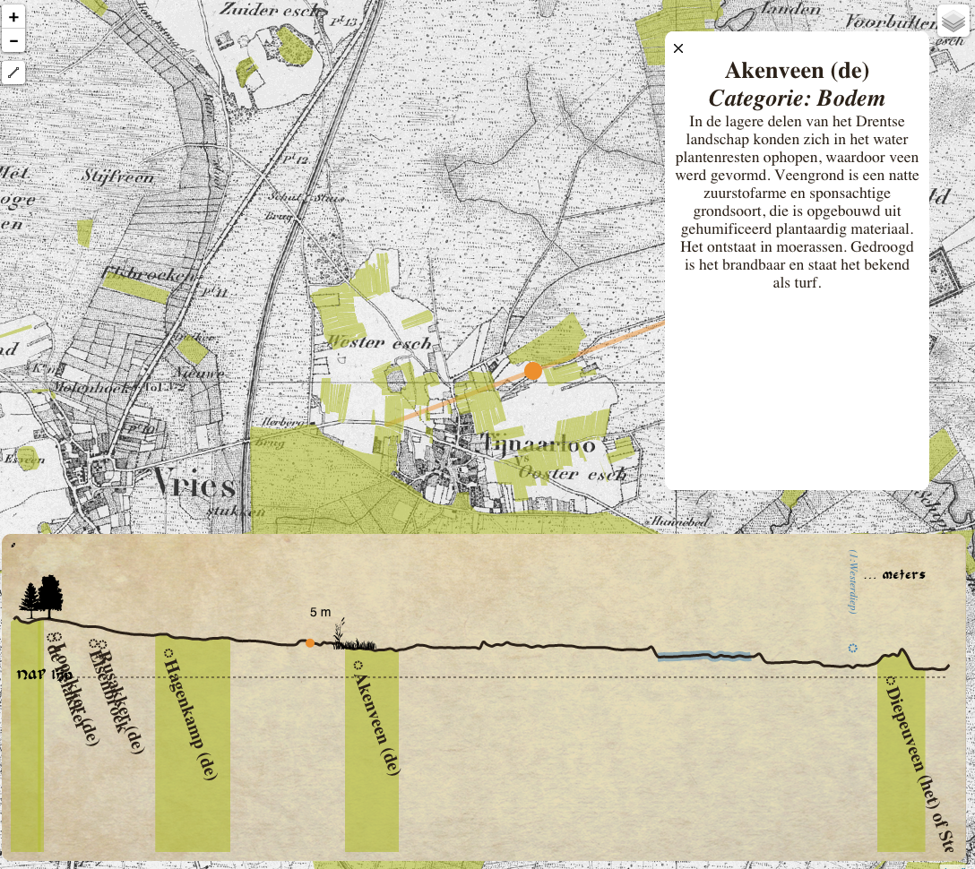
The figure 16 shows the drop-down panel with multiple background layers. If the user mover the mouse over the drop-down menu this will appear. Then they can click on the preferred layer. The image after that shows the information panel that will appear when the mouse moves over one of the fields. The name and category of the field is given, with some supplementing information if available.

The user can click on the line button to start drawing a line.

Back-end

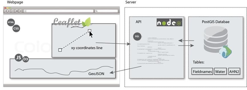
See figure 19 for the overall set-up of the back-end system.

<figure id=”method2” >

</figure>

On the web page a line can be drawn by Leaflet Draw on the Leaflet map. The coordinates of this line are edited to a line string format and parsed into a SQL query. This query is explained in appendix 9 code snippet 2 and 3. This query is asked to the API which requests the data from the PostGIS database. The response is a geoJSON array containing the heights on every 10 meters of the line (code snippet 11). This data is parsed back to the script of the website and used to draw the transect line and all the other characteristics needed.

In appendix 9 the code of the communication between the front-end and back-end is given. As well as an example of the leaflet map and the d3 compilation of the request.

The total code can be found on https://github.com/NieneB/veldnamen.

The database contains the following data:

• Field-names polygons with the names and categories
• Raster with AHN height data
• Water bodies with their names, polygons

Results Sub-objective 3. Evaluating the web-application

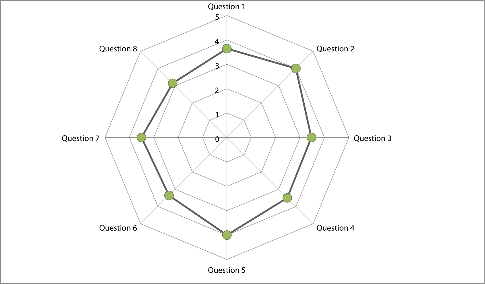
14 people were asked to use the application and fill in the small questionnaire. The graph below shows the average outcome per question. With 2 and 5 being the most positive and 8 being the most negative. Overall the scores are quite high.

Question 2 was if people were triggered to perform multiple actions was answered the most positive. Also question 5; if the user found the information surprising and interesting, scored high. Meaning that the application was perceived interesting and the user lingered around to discover more.

Question 8; everything was working as expected, got the lowest score; the functionality did not work as the user would expect.

On average the user requirements scored a 3.66. The functional requirements scored a 3.32.

For the total answer overview see appendix 13 and the extra remarks made in appendix 14.

Discussion

The short time span (4 months) to conduct the research, resulted in a product that is not finished completely. Only a rough prototype was produced. Because the conducting researcher did all steps of the process herself, this resulted in time shortage and a lack of specific technical skills and knowledge. The iterative process of a good design oriented research, had to be followed several times in order to come to a user centred design with a technical working application. Recommended would be to outsource certain parts of the development of an application to professionals with specific aimed skills. Overall, the first results were promising and the main idea came forth from the results.

Per sub-objective the discussion will be given.

Discussion Sub-objective 1. The design requirements

Not much time was invested in specifying the design objectives and requirements. No research was conducted into the target group.

Discussion on the data

The data was provided by the RCE, because this all came in an unknown file structure with no meta-data behind the various datasets, the background and quality of the data taken into consideration for this research. Also the categorization of the names, without a category assigned yet, was done in a harsh and crude way. A simple sting comparison was done, which also resulted in wrong assigning of categories. For example short words like val and gat could also appear in names which didn’t refer to this particular relief structure. Also the order of the script which starts at the beginning of the table and runs on the order of categories through the possible categories, resulting in more use of names in the category of altitude and forests, then the last category wind direction and miscellaneous. The order of the table and so the order of running the script can be seen in appendix 4 . Overall no human cognition came to pass for the process, which makes the classification crude. But the focus was more on the technical development of the application then the correctness of the background information.

The professional knowledge about the data was with the RCE; therefore the focus was more on the visualization and not improving the information in the data. A lack of professional knowledge about the field-names was kept at a low level.

On the other hand the correspondence between the AHN and the field-names can be discussed for the height is the recent height, while the fields originate from 1800. The question lingers if the altitude difference is still the same as in 1830? A lot could have changed since. The same is valid for the water topologies and the different background maps used. Which all originate from 2015. Therefore they do not show the correct correlation with the field names. Some lakes disappeared and new ones appeared. The same as train and road tracks. The default background map is a map from 1830, showing a good reference for the field-names. But on the transect line, water bodies show up that cannot be seen on this base layer. When switching to the base layer from the current map, the water bodies do correlate but the field-names are not referenced.

Discussion Sub-objective 2. Building the prototype web-application

Data exploration gave multiple ideas; no testing was done which idea would prove the best results. Solely made on personal preferences.

Front-end

The theoretical framework did bring in some nice techniques that are found back in the application. Like the brushing and linking techniques. However when it comes to colour, patterns, symbol or size selection it was more done in a subjective manner then looking at the theory. It is hard to follow a strict theoretical framework and every visualization and story to be told is an individual case. and so, needs to be designed and created individual.

Geo-visualization is so broad and there are so many ways in which a dataset can be described that it is not possible to set up a framework in steps to follow. For the field-names there are probably a variety of forms to present them. From simply displaying the names on a map, to animated dynamic maps.

Back-end

The technology to build the web application was a restricting factor in the implementation of some ideas. For example, displaying the total length of the line was a hard technical trick and therefore not finished or worked out. Also the panel with the extra base-layers was supposed to show all the time. But the plug-in for the miniMap did not support this and there was no time to work around it. On the positive site, the D3 package provided good and simple ways to work with the graphical display of the transect line. It is an easy tool and draws simple SVG formats in the browser with the possibility to animate it easily. Also leaflet proved to be quick and simple, providing the basic needs for a map and displaying the geoJSON of the field-names on it. The drawing plug-in was also easily edited so only the possibility for drawing a line was enabled. Though, changing the text from English to Dutch was harder and therefore also not implemented in the short time span. Still some minor defaults can be noticed but the overall picture shows a good first idea of the application.

The database and API slow down the process of plotting the transect line. The AHN data is too detailed for every 10 meters a point is asked to intersect. This makes the process really slow, especially when long lines are requested.

Discussion Sub-objective 3. Evaluating the web-application

Though, after the first concept of the application, the time was not found to conduct a good testing round and adjust the application to this. The advice and comments received in the end, where very useful and showed clearly where the user got stuck. Though, there was no time to implement this anymore.

The test with the questionnaire was conducted very quickly and not thoroughly. The statements posed may be too positively asked. 5 levels might be giving the people an opportunity of choosing 3 which is too neutral. The participants were biased and influenced by that they like heritage and understand the project in the bigger picture. More participants were needed and in the target group description.

Overall the application was perceived attractive and beautiful. As the scores of the questionnaire are on the positive side. The functionality scored the lowest as the user requirements scored slightly higher.

Conclusion

Although the overall time span of the project was too short, a first prototype application was developed. This already shows the potential of explaining the field-names in correlation to its direct environment. There are many more possibilities of visualization to tell the same story. But one type of story had to be selected to tell and develop. If this was the best way to tell the story of the field-names can only be tested if multiple visualizations are developed and compared. Every geo-visualization needs to be looked at individually and developed specifically for the story it needs to tell. There are many recommendations to be done on the technical and design part of the prototype. The next section shows some ideas and comments that can easily be implemented when more time was available.

Recommendations on the application

There are sufficient recommendations to be done to improve the web application. Some are extra ideas, that didn’t receive the time to be implemented yet and others are recommendations done by the test group.

One idea was split the overall layout of the web-page, up in 3 screen parts. First a screen with information, then scroll through to the next screen, where the user can draw a line. If the line is loaded, a new screen is show with the transect line and the information behind it. If the user wants to go back to either the explanation, or drawing a new line, they can simply scroll up and start over again. This form of websites is called a carousel and starts to become more popular.

An essential thing to be added is a waiting sign. Because the application is rather slow, and the user doesn’t see a waiting sign yet. The user experiences this now as nothing is happening after their actions. The user they need to know that something is happening and will soon get a reward.

Overall, the information in form of text was not complete. More specific stories behind the field-names are needed to make it more interesting. Also, images, indicating vegetation types, soil types or any other object related to the field-names, are missing. It will make the transect-line more interesting and appealing.

Some other small recommendations are:

• The map and transect line need scale indication.
• Make the application suitable for multiple browsers.
• Make the extra map layers always visible in front.
• Find water body data from 1830 instead of 2015.
• For user investment, let the user draw a field and add a field-names they know, themselves.
• Make the water bodies more ecstatically correct, by lowering them beneath the ground-level and fill with blue.

References

Appendix

Annex 1. R script converting files to shape-file.

filenames <- list.files()
filenames <- list.files(filenames , pattern = "*.TAB" ,full.names = T)

x = list of folder files # cat = category folder
exportToShape <- function(x, cat){
  for(i in 1:length(x)){
      name <- x[i]
      nr <- strsplit(name, "/")
      layer <- substr(nr[[1]][2], 1, nchar(nr[[1]][2])-4 )
      lemming <- substr(nr[[1]][2], 4, nchar(nr[[1]][2])-4)
      file <- readOGR(name, layer)
      file$category <- cat
      file$lemming <- lemming
      writeOGR(obj = file, dsn = "shape_vlak", layer = layer, driver = "ESRI Shapefile", overwrite_layer = T)
  }
}
exportToShape(filenames, "overig")

Annex 2. SQL adjustments field-names

-- UPDATE veldnamen3 SET naam = naam_2 WHERE naam IS NULL;
-- UPDATE veldnamen3 SET atoto_co_3 = code_3 WHERE atoto_co_3 IS NULL;
-- UPDATE veldnamen3 SET atoto_co_2 = code_2 WHERE atoto_co_2 IS NULL;
-- DELETE FROM veldnamen3 WHERE naam IS NULL;
-- ALTER TABLE veldnamen3 DROP COLUMN naam_2 CASCADE;
-- ALTER TABLE veldnamen3 DROP COLUMN code_1_ CASCADE;
-- ALTER TABLE veldnamen3 DROP COLUMN code_2 CASCADE;
-- ALTER TABLE veldnamen3 DROP COLUMN code_3 CASCADE;
-- ALTER TABLE veldnamen3 DROP COLUMN code_4 CASCADE;
-- ALTER TABLE veldnamen3 RENAME COLUMN atoto_co_1 TO code_1;
-- ALTER TABLE veldnamen3 RENAME COLUMN atoto_co_2 TO code_2;
-- ALTER TABLE veldnamen3 RENAME COLUMN atoto_co_3 TO code_3;

Annex 3. R script detecting categories

library(sp)
library(raster)
library(rgdal)
library(rgeos)
require(RPostgreSQL)
require(rgdal)

swd("/Users/waag/Documents/MGI_Stage/9_veldnamen/10_VeldnamenOrgineel/")

# csv alle categorien en Lemmings
categorie <- read.csv(file = "Categorie_Alles.csv", header = T , sep=","   )

# shape-file alle velden + namen
velden <- readOGR(dsn = "/Users/waag/Documents/veldnamen.shp", layer = "veldnamen", stringsAsFactors = F)

# write shape-file back
writeOGR(obj = velden, dsn = "veldnamen_cat.shp", layer = "veldnamen_cat", driver = "ESRI Shapefile")

# modifying shape-file
velden$CODE_1[velden$CODE_1 != NULL] <- velden$ATOTO_CODE
## correctie
velden$CODE_1[velden$CODE_1 == "D02"] <- "D2"
velden$CODE_1[velden$CODE_1 == "E04"] <- "E4"
velden$CODE_1[velden$CODE_1 == "G03"] <- "G3"
velden$CODE_1[velden$CODE_1 == "B03"] <- "B3"
velden$CODE_1[velden$CODE_1 == "G06"] <- "G6"
velden$CODE_1[velden$CODE_1 == "G07"] <- "G7"
velden$CODE_1[velden$CODE_1 == "A01"] <- "A1"
velden$CODE_1[velden$CODE_1 == "D03"] <- "D3"
velden$CODE_1[velden$CODE_1 == "D06"] <- "D6"
velden$CODE_1[velden$CODE_1 == "O08"] <- "O8"
velden$CODE_1[velden$CODE_1 == "O02"] <- "O2"

## categorien toevoegen
i <- 0
j <- 0

for( i in 1:length(velden$NAAM)){
  naam <- velden$NAAM[i]
  for( j in 1:length(categorie$Lemming)){Answers on the questionnaire
    CODE <- categorie$Lemming_Code[j]
    tekst <-  paste(categorie$Lemming[j],"|",categorie$amaltertieven[j] , sep = "")
    geld <- grepl(tekst, naam, ignore.case=T)
    if(geld){
      if(is.na(velden$CODE_1[i])){
        velden$CODE_1[i] <- paste(CODE)}
      else if(is.na(velden$CODE_2[i])){
        velden$CODE_2[i] <- paste(CODE)}
    }
    print(paste(naam, tekst, CODE, geld))
  }
}

Annex 4. Categories field-names form RCE

Lemming Code	Category	Category Code	Lemming	Name Alternatives	Count first Code	Count second Code
A1	Relief	A	berg	bergen|bergje|barg	210	38
A10	Relief	A	leest		13	247
A11	Relief	A	richel		1	14
A12	Relief	A	duin	dun|dunne	39	22
A13	Relief	A	dal	daal|del|dil	39	175
A14	Relief	A	kuil	koel	18	4
A15	Relief	A	waard	weerd	2	8
A16	Relief	A	kwab	kweb|kwebbe|kwabbe	4	10
A17	Relief	A	gat		11	8
A18	Relief	A	put
A19	Relief	A	laag	laagen|laagte|leeg|lege	1	44
A2	Relief	A	bult	bulten|bulte|bultje|bultien	48	15
A20	Relief	A	val		499	53
A21	Relief	A	plat
A22	Relief	A	vlak	vlakte|vlakkien		2
A23	Relief	A	hol		15	120
A24	Relief	A	glij	glijt|gleet|gleed	2	16
A3	Relief	A	hoog	hoge|hoogte|heugt	71	41
A4	Relief	A	hoorn	Horne|hörne|heurn	64	17
A5	Relief	A	hel	helle	33	62
A6	Relief	A	hul	hulle	7	1
A7	Relief	A	pol		2	39
A8	Relief	A	hoop		2
A9	Relief	A	nor	norre	31
B1	Bodem	B	zand	sand	80	36
B10	Bodem	B	grijs	grijze|grauw
B11	Bodem	B	ele		1	5
B12	Bodem	B	bruin	bruun
B2	Bodem	B	leem		3	2
B3	Bodem	B	veen		279	175
B4	Bodem	B	klei		15	122
B5	Bodem	B	steen	stien|stein	88	39
B6	Bodem	B	kei	kai|kaai	2
B7	Bodem	B	zwart		10	11
B8	Bodem	B	wit		46	44
B9	Bodem	B	rood	rode	27	32
C1	Watermen	C	meer	meren	88	28
C10	Watermen	C	wiel	waal	1	1
C11	Watermen	C	zee			3
C12	Watermen	C	vals	valsch
C13	Watermen	C	weier	weiert|weijert	1	4
C14	Watermen	C	veentje	veentie		3
C2	Watermen	C	poel		19	16
C3	Watermen	C	dobbe		14	3
C4	Watermen	C	streng		33	6
C5	Watermen	C	diep		15	24
C6	Watermen	C	beek	beeck	18	14
C7	Watermen	C	water		4
C8	Watermen	C	kolk		6	10
C9	Watermen	C	leek
D1	Beekdal_Moeras	D	broek	broeken|broekje	416	221
D10	Beekdal_Moeras	D	gagel
D11	Beekdal_Moeras	D	moor	moer|moerde	1
D12	Beekdal_Moeras	D	goor	gor		33
D13	Beekdal_Moeras	D	sleek	slijk
D14	Beekdal_Moeras	D	rus	rusch	3	6
D15	Beekdal_Moeras	D	geel	gele	5	28
D16	Beekdal_Moeras	D	slob	slom
D17	Beekdal_Moeras	D	eis		1	8
D18	Beekdal_Moeras	D	schol	scholte|school|schel	6	15
D19	Beekdal_Moeras	D	sek	sekke
D2	Beekdal_Moeras	D	maat	made|maad|maadje	350	246
D3	Beekdal_Moeras	D	mars		18	24
D4	Beekdal_Moeras	D	vledder	vleer|vlier|fleer|flier	25	15
D5	Beekdal_Moeras	D	stroet	stroot|stroe	13	5
D6	Beekdal_Moeras	D	hem	ham	56	19
D7	Beekdal_Moeras	D	horst	hurst	23	7
D8	Beekdal_Moeras	D	oel		1	5
D9	Beekdal_Moeras	D	riet	reit|raait|reet	8	8
E1	Bossen	E	loo		1572	63
E10	Bossen	E	haag	hagen|heeg|heg		44
E11	Bossen	E	els	elze|eller|elder	20	14
E12	Bossen	E	hulst	huls
E13	Bossen	E	den	denne	118	582
E14	Bossen	E	esch|asch		59	61
E15	Bossen	E	wilg	ween|wene|wede|wee|warff|warve|werff|werv	7	7
E16	Bossen	E	eik	eek|ekkel|eck	1	37
E17	Bossen	E	hazel	hessel
E18	Bossen	E	struik	stroek	1
E19	Bossen	E	bramen	brummel		10
E2	Bossen	E	hees	heeze|heze	75	20
E20	Bossen	E	meidoorn	hageldoorn		2
E21	Bossen	E	doorn		775	47
E22	Bossen	E	bosbes	kreus|kreuzen|krös|krözen
E23	Bossen	E	zwartebosbes|blauwebosbes	bliek|blik		5
E24	Bossen	E	bessen		1
E25	Bossen	E	roos	rosen|rozen
E26	Bossen	E	stok	stock
E3	Bossen	E	stobbe	stob	61	40
E4	Bossen	E	bos	bosch|busch	251	136
E5	Bossen	E	hout		48	29
E6	Bossen	E	holt		120	12
E7	Bossen	E	laar		9	8
E8	Bossen	E	wold	woold	2	20
E9	Bossen	E	strubbe		10	37
F1	Veldgrond_stuifzand	F	veld	velt	162	112
F10	Veldgrond_stuifzand	F	lijsterbes	kweekeboom
F2	Veldgrond_stuifzand	F	heide	heide|heet|hiet	23	8
F3	Veldgrond_stuifzand	F	haar	hare	33	20
F4	Veldgrond_stuifzand	F	zuring		2	2
F5	Veldgrond_stuifzand	F	woest		4	3
F6	Veldgrond_stuifzand	F	wild	wilden|wildernis	1	4
F7	Veldgrond_stuifzand	F	ruig	roege	4	5
F8	Veldgrond_stuifzand	F	brem	braam|broam|breem|bram	1	1
F9	Veldgrond_stuifzand	F	wind		2	8
G1	Wilde_dieren	G	fazant|patrijs	hunder|hoender|hoonder	29	15
G10	Wilde_dieren	G	valk		12
G11	Wilde_dieren	G	kraanvogel	kraan|krane|craan|crane		1
G12	Wilde_dieren	G	reiger
G13	Wilde_dieren	G	mus
G14	Wilde_dieren	G	raaf	raven	14
G15	Wilde_dieren	G	duif	duiven|duven|doef|doeven	2
G16	Wilde_dieren	G	mees	meeze
G17	Wilde_dieren	G	ooievaar	ooievaar|heileuver|ooievaar|eiber|scholbos|luibert	1
G18	Wilde_dieren	G	kraai		2
G19	Wilde_dieren	G	spreeuw	spree
G2	Wilde_dieren	G	haan	hane	13	20
G20	Wilde_dieren	G	hond	hund	2	1
G21	Wilde_dieren	G	kat		4	1
G22	Wilde_dieren	G	bever			1
G23	Wilde_dieren	G	vos		5	4
G24	Wilde_dieren	G	wolf	wolven	10	10
G25	Wilde_dieren	G	haas	hazen	11	11
G26	Wilde_dieren	G	konijn		9	5
G27	Wilde_dieren	G	otter		1	2
G28	Wilde_dieren	G	das		1	1
G29	Wilde_dieren	G	adder	edder	7	32
G3	Wilde_dieren	G	uil	oel	4	9
G30	Wilde_dieren	G	mug		1	1
G31	Wilde_dieren	G	luis	luizen	2
G32	Wilde_dieren	G	bij	iemen|ymen|yemen	24	4
G33	Wilde_dieren	G	bloedzuiger	egel|iegel
G34	Wilde_dieren	G	aal	alen	3
G35	Wilde_dieren	G	vis	visch	6	6
G4	Wilde_dieren	G	ekster	aakster|okster
G5	Wilde_dieren	G	kievit	kiewiet|kieft|Kieviet	6	6
G6	Wilde_dieren	G	eend	ent	9	3
G7	Wilde_dieren	G	gans	ganzen|gaans|gaanzen|goos|gozen|goes	2	3
G8	Wilde_dieren	G	snip
G9	Wilde_dieren	G	leeuwerik
O1	Overig	O	sassen
O10	Overig	O	wed	wet	32	38
O11	Overig	O	dansel
O12	Overig	O	walg		1	2
O13	Overig	O	alk	halk
O14	Overig	O	hartzeer
O15	Overig	O	buis
O16	Overig	O	helmer			1
O17	Overig	O	staart		3	5
O18	Overig	O	vlas		4
O2	Overig	O	bol		21	20
O3	Overig	O	viool	violen
O4	Overig	O	distel	dissel|diesel
O5	Overig	O	bloem			8
O6	Overig	O	ronsel		18
O7	Overig	O	mos		3	3
O8	Overig	O	klaver		2	22
O9	Overig	O	groen		1	3
W1	Wind	W	oost	ooster	121	33
W2	Wind	W	noord	noorder	25	18
W3	Wind	W	west	wester	8	20
W4	Wind	W	zuid	zuider	11	44

Annex 5. Leaflet map initializing

var basemaps ={ 
  "_1830": L.tileLayer("http://s.map5.nl/map/gast/tiles/tmk_1850/EPSG900913/{z}/{x}/{y}.png" ),
  "_2015": L.tileLayer("http://{s}.tile.openstreetmap.org/{z}/{x}/{y}.png"),
  "Hoogte": L.tileLayer("http://s.map5.nl/map/gast/tiles/relief_struct/EPSG900913/{z}/{x}/{y}.jpeg")
};

var map = new L.map("map", {
  maxZoom: 15,
  minZoom: 12,
  layers: basemaps._1830
});

map.setView([53.079529, 6.614894], 14);
map.setMaxBounds([
  [52.861743, 6.458972],
  [53.202277, 6.958035]
]);

Annex 6. AHN pre-processing

AHN2 from the research area

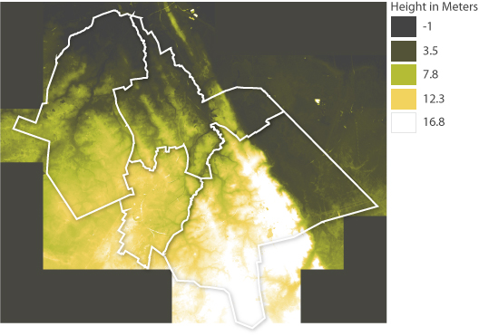
The AHN2 tiles covering the research area were downloaded from nationaalgeoregister.nl to show the relation of the field-names with the environment. The AHN has proved useful for historical research. Small differences in the landscape can be seen in the AHN2 and already historians and archaeologist use it to discover old settlements that can’t be discovered with the naked eye. (Actueel Hoogtebestand Nederland, n.d.)The AHN is measured with laser altimetry or LIDAR. Laser beams shot from an airplane and localized with GPS. It is measured over several time periods and merged in the end to get a detailed measurement of the height. The eventual end product delivered is corrected to ground level.(maaiveld) So vegetation, buildings and other object do not appear. (Actueel Hoogtebestand Nederland, n.d.) These filtered areas are given no-data values. The raster data has a resolution of 5 meters and a precision of systematic and stochastic error of max 5 cm the projection is RD new ( EPSG28992). (Actueel Hoogtebestand Nederland, n.d.) The maximum and minimum values of the total area are 29.5 and -1.9 meters respectively.

AHN tiles downloaded:

ahn2_5_07cz1.tif	ahn2_5_12en1.tif
ahn2_5_07cz2.tif	ahn2_5_12en2.tif
ahn2_5_07dz1.tif	ahn2_5_12ez1.tif
ahn2_5_07dz2.tif	ahn2_5_12ez2.tif
ahn2_5_11fz2.tif	ahn2_5_12fn1.tif
ahn2_5_12an1.tif	ahn2_5_12fn2.tif
ahn2_5_12an2.tif	ahn2_5_12fz1.tif
ahn2_5_12az1.tif	ahn2_5_12fz2.tif
ahn2_5_12az2.tif	ahn2_5_12gn1.tif
ahn2_5_12bn1.tif	ahn2_5_12gn2.tif
ahn2_5_12bn2.tif	ahn2_5_12gz1.tif
ahn2_5_12bz1.tif	ahn2_5_12gz2.tif
ahn2_5_12bz2.tif	ahn2_5_12hn1.tif
ahn2_5_12cn1.tif	ahn2_5_12hn2.tif
ahn2_5_12cn2.tif	ahn2_5_12hz1.tif
ahn2_5_12cz1.tif	ahn2_5_17bn2.tif
ahn2_5_12cz2.tif	ahn2_5_17en1.tif
ahn2_5_12dn1.tif	ahn2_5_17en2.tif
ahn2_5_12dn2.tif	ahn2_5_12en1.tif
ahn2_5_12dz1.tif	ahn2_5_12en2.tif
ahn2_5_12dz2.tif	ahn2_5_12ez1.tif
ahn2_5_12fn1.tif	ahn2_5_12ez2.tif

For use in the application, the transect line looks best when not containing any gaps. Therefore, the no-data values are filled by the fill no-data tool of Qgis. This takes an average of around 100 pixels to calculate the average height of the missing pixels.

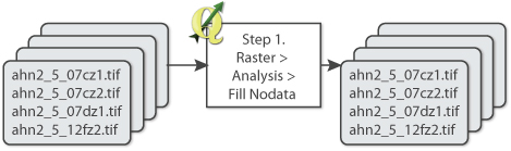
Annex 7. Water topologies pre-processing

The water bodies are downloaded from the open data PDOK.nl. The Top10NLactueel contains all topology of the Netherlands on a scale of 1:25.000. From this dataset only the water polygons are used and clipped to the research area. So the names of the water bodies can be included into the application. (“TOP10NL | Publieke Dienstverlening Op de Kaart Loket,” n.d.) All in EPSG28992.

Map sheets Top10NL downloaded

Top10NL_17O

Top10NL_1rW

Top10NL_1rO

Top10NL_1rW

Annex 8. Loading data into the PostGIS database

Loading data into the database

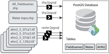
Loading data in the database

Shp2pgsql
➜  ~ shp2pgsql -s 28992 /<path name> /veldnamen.shp veldnamen | psql -U user -d veldnamen
    
Raster2pgsql
➜  ~ raster2pgsql -s 28992 -I -C /<path name>/ahn2*.tif public.ahn2 | psql -d veldnamen

Annex 9. Request & Response for transect line

D3 request coordinates and drawing transect path

d3.json("transect?linestring=" + coordinates, function(json){
  console.log("requesting line from database");
  console.log(json)
  var line = d3.select("#line")
  line.selectAll(".transect")
  .data(linestring)
  .enter()
  .append("path")
  .attr("class", "transect")
  .attr("d", lineFunction(json))
  .attr("stroke", "#2B2118")
  .attr("stroke-width", 3)
  .attr("fill", "none");
});

After a line is drawn on the Leaflet map with Leaflet Draw, the coordinates of the line are inserted into the request ($1) as a LINESTRING format. The line is in WGS84 (EPSG4326) and needs to be converted to RDNew (EPSG28992) in order to extract the location with the other data at the right location.

Request & Response for transect line

app.get("/transect", function (req, res) {
  query(queries.transect, ["LINESTRING (" + req.query.linestring + ")"] , function(err, result) {
    if (err) {
    res.status(500).send(err);
    } else {
    res.send(result.rows.map(function(row) {
      row.geometry = JSON.parse(row.geometry);
      return row;
    }));
    }
  })
});

The line

WITH line AS
  -- Create line geometry
  (SELECT ST_Transform(ST_GeomFromText($1 , 4326), 28992) AS geom),

The line is then cut into parts of 10 meter and points are generated with its percentage location along the line.

Point and percentage at every 10 meter along the line

linemesure AS
  (SELECT ST_AddMeasure(line.geom, 0, ST_Length(line.geom)) as linem,
  generate_series(0, ST_Length(line.geom)::int, 10) as i
  FROM line),

points2d AS
  (SELECT ST_GeometryN(ST_LocateAlong(linem, i), 1) AS geom, (i*100/ST_Length(linem)) as percentage
  FROM linemesure),

This array of points is intersected with the AHN table to ext rat the height value for every point.

Get height per point

AHN AS
  -- Get DEM elevation for each
  (SELECT p.geom AS geom, ST_Value(ahn.rast, 1, p.geom) AS heights, percentage
    FROM ahn, points2d p
    WHERE ST_Intersects(ahn.rast, p.geom)),

Also the points are intersected with the field names table to see if a points falls into a field, and which name and category code it belongs to.

Get field-name for intersecting points

fields AS
  (SELECT naam AS naam, code_1_ AS category1, code_2 AS category2, ST_Intersection(p.geom, veldnamen2.geom) AS geoms
  FROM veldnamen2, points2d p 
  WHERE ST_Intersects(veldnamen2.geom, p.geom)),

Then the points are intersected with the water topology table to see if a points falls into a water body, and which name and category code it belongs to.

Get field-name for intersecting points

--Get Water intersects
waters As
  (SELECT naamnl AS waternaam, typewater AS typewater, identifica AS waterId, ST_Intersection(p.geom, water.geom) AS geomz
  FROM water, points2d p
  WHERE ST_Intersects(water.geom, p.geom)),

In the end all point that fall into a field or water body are joined to the total amount of points to contain the whole range of points.

Join all outcomes

points AS
(SELECT *  FROM AHN LEFT OUTER JOIN fields ON (AHN.geom = fields.geoms)),

points1 AS
(SELECT * FROM points LEFT OUTER JOIN waters ON (points.geom = waters.geomz))

This is all send back as one complete GeoJSON response.

final GeoJSON response

-- Make points:
SELECT ST_AsGeoJSON(ST_MakePoint(ST_X(ST_Transform(ST_SetSRID(geom, 28992),4326)), ST_Y(ST_Transform(ST_SetSRID(geom, 28992),4326)), heights)) 

AS geometry, naam, heights, percentage , category1, category2, waternaam, typewater, waterID
FROM points1

Eventually the response of the request will be a GeoJSON. An example of the GeoJSON array is shown below.

Example GeoJSON response

[
  {
    "geometry": {
      "type": "Point",
      "coordinates": [
        6.6089395293246,
        53.0818691708253,
        8.05700016021729
      ]
    },
    "naam": "Zuurpol (de)",
    "heights": 8.05700016021729,
    "percentage": 0.826035566357403,
    "category1": "A1",
    "category2": null,
    "waternaam": null,
    "typewater": null,
    "waterid": null
  },
  {…},
  {…},
  {
    "geometry": {
      "type": "Point",
      "coordinates": [
        6.62981923722014,
        53.0856490864126,
        4.8439998626709
      ]
    },
    "naam": "Gryze Steen",
    "heights": 4.8439998626709,
    "percentage": 55.5813292359005,
    "category1": null,
    "category2": null,
    "waternaam": null,
    "typewater": "meer, plas, ven, vijver",
    "waterid": "NL.TOP10NL.128375900"
  },
  {…},
]

Annex 10. Questionnaire for testing the application

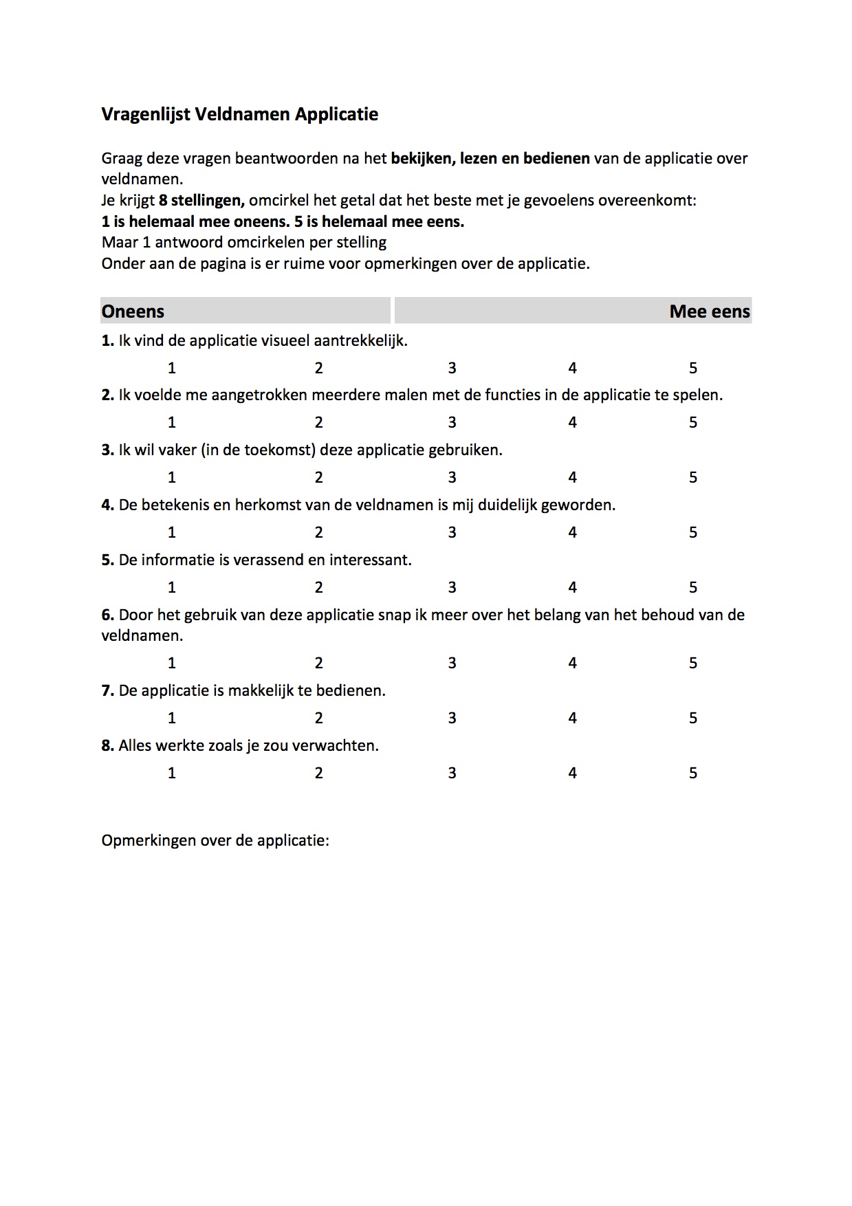
Annex 11. Mood board

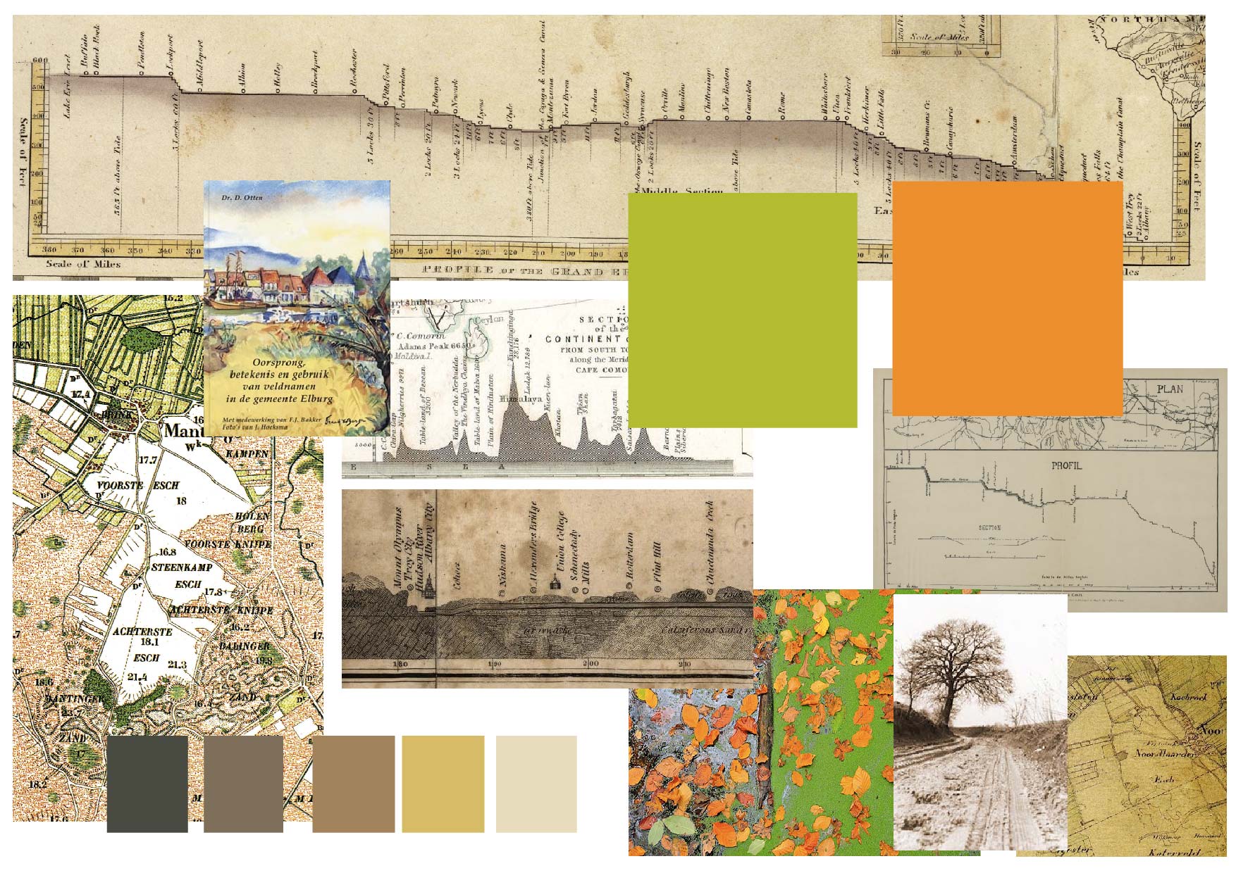
Annex 12. Variations on the main idea

For also on this main idea some variations can be made, these will be listed here.

• Soil properties as colours of the fields. Or pattern of the specific soil type. Like stones, clay, sand etc. Giving colours or patterns to the fields according to the soil property. Like a Stonefield or Redfield.
• Pop-ups with explanations and texts. Linking field-names to textual explanation, adding pictures of the surroundings and landscape characteristics. Vegetation types, animal occurrence.
• Adding pictures or symbols of vegetation types and animals on the transect line. As well as houses to indicate towns and cities. Water bodies as blue dips in the transect line. Give more explanation per category or field-name type. Include pictures of trees, shrubs, plants or animals with which the field-name is connected.
• Creating a small 3D landscape by adding multiple transect lines, stacked in front of each other.
• Link stories provided to the line, so pop-ups with provided stories from the book.

Annex 13. Answers on the questionnaire

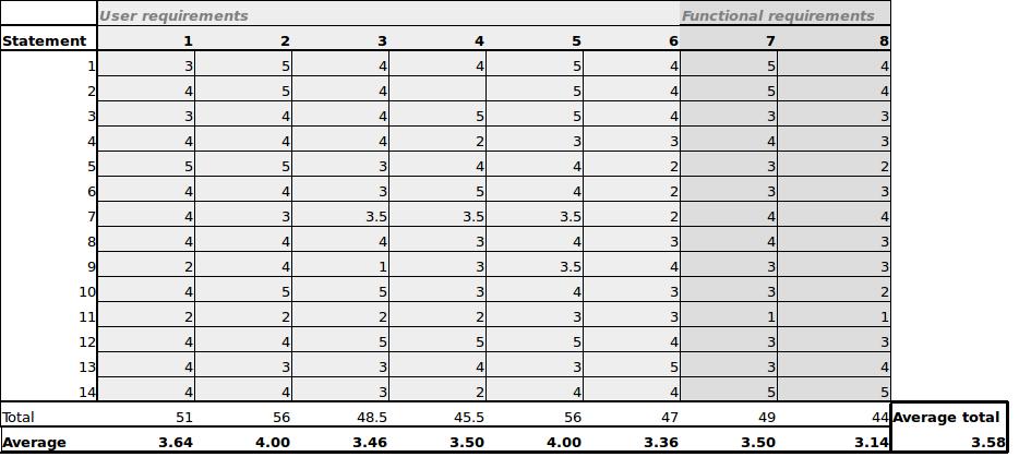
Annex 14. Remarks on the questionnaire

• Works logical, though information is missing.
• Make the pop-up disappear when the mouse moves away.
• I miss a total overview of the page.
• Finish line, not working..
• The elevation graph should follow the x,y of mouse instead of following just x.
• Text window sometimes conflicts with the layer selector.
• Cursor on the map synchronises with the moving circle on the line.
• Also point selection, not only line.
• Ugly button on the introduction page.
• I would like to know more about the different map layers.
• Drawing button for the line is hard to find.
• While waiting, put a waiting sign.
• You would expect the information about the field to pop up when the moving circle is on the field, instead of the mouse.
• Ask people for collaboration, for example make a text-editor do the texts.
• Typography was hard to read.
• A lot of introduction text.
• Looks like the focus is more on the height then on the names.
• Drawing the line and clicking was difficult, had to get used to it. Nice view into height differences. Though I don’t understand the origin of the field names yet. The line shows weird peaks, I would like to know what this is.
• I would like to have this for the area I live in.
• With long lines, the names are on top of each other.
• Clicking last point of the line to finish it was difficult to find.
• Nice that you really learn something about the names through the information.
• Put the year on the map.
• Some targeted assignments would help understanding the field-names better.
• Nice, I would like to have this were I am personally living.
• More locations would be nice.
• Layout of the map is nice, but some this could be made more readable.
• Continue!
• Unpredictable behaviour with drawing the line.
• Can’t get the results good on the screen.
• Text at the bottom is not readable.

References

Actueel Hoogtebestand Nederland. (n.d.). AHN - Actueel Hoogtebestand Nederland - homepage [overzichtspagina]. Retrieved July 13, 2015, from http://www.ahn.nl/index.html
Bertin, J. (2000). Matrix theory of graphics. Information Design Journal, 10(1), 5–19.
Blok, C. (2000). Monitoring Change: Characteristics of Dynamic Geo-spatial Phenomena for Visual Exploration. Spatial Cognition II, 1 (2000), 16–30. http://doi.org/10.1007/3-540-45460-8_2
Cartwright, W., Miller, S., & Pettit, C. (2004). Geographical visualization: Past, present and future development. Journal of Spatial Science, 49(1), 25–36. http://doi.org/10.1080/14498596.2004.9635003
Cerasuolo, F., Cutugno, F., & Leano, V. A. (2012). Visualization with a New Visual Metaphor for Hierarchical and Stratified Temporal Domain. In S. D. Martino, A. Peron, & T. Tezuka (Eds.), Web and Wireless Geographical Information Systems (pp. 57–71). Springer Berlin Heidelberg. Retrieved from http://link.springer.com.ezproxy.library.wur.nl/chapter/10.1007/978-3-642-29247-7_6
Deal, L. (2014). Visualizing Digital Collections. Technical Services Quarterly, (April), 30–30. http://doi.org/10.1080/07317131.2015.972871
DEN. Home. (n.d.). Retrieved May 6, 2015, from http://www.den.nl/
Dibiase, D., Maceachren, A., Krygier, J., & Reeves, C. (1992). Animation and the Role of Map Design in Scientific Visualization. Cartography and Geographic Information Systems, 19(4), 201–&. http://doi.org/10.1559/152304092783721295
Droj, G. (2010). Cultural Heritage Conservation by GIS, 1–6.
Elwood, S. (2011). Geographic Information Science: Visualization, visual methods, and the geoweb. Progress in Human Geography, 35(3), 401–408. http://doi.org/10.1177/0309132510374250
Erfgeo. (n.d.). Retrieved July 22, 2015, from http://erfgeo.nl/
Erfgoed & Locatie (n.d.). Retrieved July 22, 2015, from http://erfgoedenlocatie.nl/
Hahmann, S., & Burghardt, D. (2013). How much information is geospatially referenced? Networks and cognition. International Journal of Geographical Information Science, 27(6), 1171–1189. http://doi.org/10.1080/13658816.2012.743664
Karavia, D., & Georgopoulos, A. (2013). Placing Intangible Cultural Heritage. Researchgate.Net, 675–678. http://doi.org/10.1109/DigitalHeritage.2013.6743815
Köbben, B., & Yaman, M. (1996). Evaluating Dynamic Visual Variables. In Proceedings of the Seminar on Teaching Animated Cartography. Madrid, Spain: International Cartographic Association. Retrieved from http://cartography.geo.uu.nl/ica/Madrid/ormeling.html
Kraak, M.-J., & Klomp, A. (1996). A Classification of Cartographic Animations: Towards a Tool for the Design of Dynamic Maps in a GIS Environment. In Proceedings of the Seminar on Teaching Animated Cartography. Madrid, Spain: International Cartographic Association. Retrieved from http://cartography.geo.uu.nl/ica/Madrid/ormeling.html
Lai, J., Luo, J., & Zhang, M. (2012). Design and Realization of the Intangible Cultural Heritage Information Management System Based on Web Map Service. Springer-Verlag Berlin Heidelberg 2012, 605–612.
Lin, H., Gong, J., & Wang, F. (1999). Web-based three-dimensional geo-referenced visualization. Computers and Geosciences, 25(10), 1177–1185. http://doi.org/10.1016/S0098-3004(99)00076-X
MacEachren, A. M., & Kraak, M.-J. (2001). Research Challenges in Geovisualization. Cartography and Geographic Information Science, 28(1), 3–12. http://doi.org/10.1559/152304001782173970
Martin, S., Reynard, E., Pellitero Ondicol, R., & Ghiraldi, L. (2014). Multi-scale Web Mapping for Geoheritage Visualisation and Promotion. Geoheritage, 6(2), 141–148. http://doi.org/10.1007/s12371-014-0102-3
Mennis, J. L., Peuquet, D. J., & Qian, L. (2000). A conceptual framework for incorporating cognitive principles into geographical database representation. International Journal of Geographical Information Science, 14(6), 501–520. http://doi.org/10.1080/136588100415710
Meyer, É., Grussenmeyer, P., Perrin, J. P., Durand, A., & Drap, P. (2007). A web information system for the management and the dissemination of Cultural Heritage data. Journal of Cultural Heritage, 8(4), 396–411. http://doi.org/10.1016/j.culher.2007.07.003
Nöllenburg, M. (2007). Geographic Visualization. In A. Kerren, A. Ebert, & J. Meyer (Eds.), Human-Centered Visualization Environments (pp. 257–294). Springer Berlin Heidelberg. Retrieved from http://link.springer.com/chapter/10.1007/978-3-540-71949-6_6
Ogao, P. J., & Kraak, M.-J. (2002). Defining visualization operations for temporal cartographic animation design. International Journal of Applied Earth Observation and Geoinformation, 4(1), 23–31. http://doi.org/10.1016/S0303-2434(02)00005-3
Ormeling, F. (1996). Teaching Animated Cartography. In Proceedings of the Seminar on Teaching Animated Cartography. Madrid, Spain: International Cartographic Association. Retrieved from http://cartography.geo.uu.nl/ica/Madrid/ormeling.html
Petrescu, F. (2007). the Use of Gis Technology in Cultural Heritage. October, (October), 1–6.
Shedroff, N. (1999). Information interaction design: A unified field theory of design. Information Design, 267–292.
Spek, T., Elerie, H., & Kosian, M. (2009). Van Jeruzalem tot Ezelakker, Levende veldnamenatlas van de Drentse Aa. Matrijs.
Steiniger, S., & Hunter, A. J. S. (2013). The 2012 free and open source GIS software map – A guide to facilitate research, development, and adoption. Computers, Environment and Urban Systems, 39, 136–150. http://doi.org/10.1016/j.compenvurbsys.2012.10.003
Tensen, T. (2014). Master Thesis Geo-data animations in television journalism :, 1–87.
TOP10NL Publieke Dienstverlening Op de Kaart Loket. (n.d.). Retrieved July 13, 2015, from https://www.pdok.nl/nl/producten/pdok-downloads/basis-registratie-topografie/topnl/topnl-actueel/top10nl
UNESCO (2003) Culture Sector - Intangible Heritage - CONVENTION FOR THE SAFEGUARDING OF THE INTANGIBLE CULTURAL HERITAGE. Paris, 17 October 20013, Retrieved May 6, 2015, from http://www.unesco.org/culture/ich/index.php?lg=en&pg=00002
Veldnamen - Encyclopedie Drenthe Online. (n.d.). Retrieved July 22, 2015, from http://www.encyclopediedrenthe.nl/Veldnamen
Verschuren, P., Hartog, R. (2005) Evaluation in Design-Oriented Research, Department of Methodology, Nijmegen School of Management, Radboud University, Nijmegen
volkscultuur. (n.d.). Retrieved May 6, 2015, from http://www.volkscultuur.nl/
Waag Society. (n.d.). Retrieved July 23, 2015, from https://www.waag.org/nl/organisatie
Zeijden, A. V. D. (2011). Immaterieel erfgoed en musea, (35), 4–6.